04. Academic writing
There are few additional aspects we have to think about for academic writing, this page covers the most important aspects of this.
Firstly, if you aren’t already using a reference manager, then you really should be! Regardless of what you use for writing, a reference manager is a very useful way of building a collection of the papers you’ve read (or plan to read…), and allows you to easily insert citations into your writing. There are lots of software available, but I’d recommend Zotero as it’s free and open-source (as all good software should be!) and it has a neat browser plugin which makes adding references to Zotero relatively painless.
I provide links to some guides for setting up Zotero in the further resources page here.
Any decent reference manager should allow you to export your references as a .bib file though, and that’s all you need to do for this.
In terms of citation style, we can use the Citation Style Language project to specify how our references should be structured. The Zotero Style Repository is a good resource to find different journal styles. Just download the one you want and add the relevant key to the YAML header:
csl: path/to/csl/file.csl
Inserting citations
So once we have our .bib file from our reference manager we just need to insert the relevant citation keys into out document.
The syntax is to wrap the citation key/s in [] and seperate reference with a ;. So an example would be:
This study found x.[@ackerman2010; @afjehi-sadat2010]
Which looks like this:
This study found x.1,2
Note that R Markdown will automatically insert a bibliography at the bottom of the document.
Cross-references
We can easily reference figures and tables using the syntax \@ref(tab:chuck-label-here) for tables or \@ref(fig:chuck-label-here) for figures.
Note that numbered sections need to be enabled for the section cross-reference to display a number.
## Example cross-references {#example-section-label}

```{r cool-table, echo=FALSE}
knitr::kable(head(mtcars), caption = "Cool table")
```

Table \@ref(tab:cool-table) shows our awesome data.

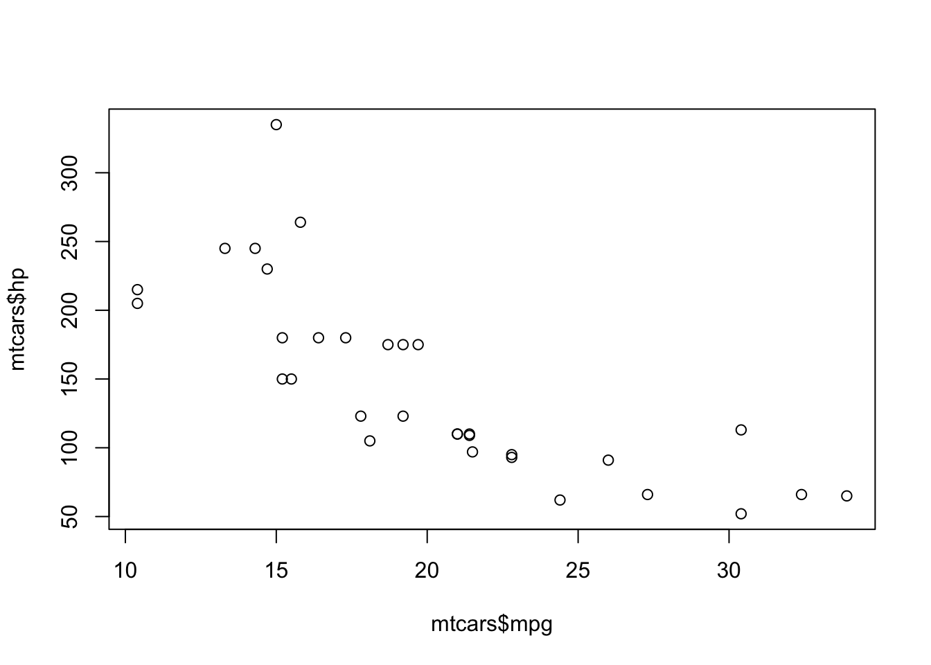
```{r cool-figure, fig.cap='Cool figure', echo=FALSE}
plot(mtcars$mpg, mtcars$hp)
```

Figure \@ref(fig:cool-figure) shows our awesome data again.

See section \@ref(example-section-label) for more info on whatever.
Which looks like this:
Example cross-references
| mpg | cyl | disp | hp | drat | wt | qsec | vs | am | gear | carb | |
|---|---|---|---|---|---|---|---|---|---|---|---|
| Mazda RX4 | 21.0 | 6 | 160 | 110 | 3.90 | 2.620 | 16.46 | 0 | 1 | 4 | 4 |
| Mazda RX4 Wag | 21.0 | 6 | 160 | 110 | 3.90 | 2.875 | 17.02 | 0 | 1 | 4 | 4 |
| Datsun 710 | 22.8 | 4 | 108 | 93 | 3.85 | 2.320 | 18.61 | 1 | 1 | 4 | 1 |
| Hornet 4 Drive | 21.4 | 6 | 258 | 110 | 3.08 | 3.215 | 19.44 | 1 | 0 | 3 | 1 |
| Hornet Sportabout | 18.7 | 8 | 360 | 175 | 3.15 | 3.440 | 17.02 | 0 | 0 | 3 | 2 |
| Valiant | 18.1 | 6 | 225 | 105 | 2.76 | 3.460 | 20.22 | 1 | 0 | 3 | 1 |
Table 1: Cool table
Table 1 shows our awesome data.

Figure 1: Cool figure
Figure 1 shows our awesome data again.
See section 2.1 for more info on whatever.
This is another area where Quarto differs slightly.
They’ve introduced a syntax for specifying the type of reference in the label so: fig-, tbl- and sec- for figure, table and sections respectively.
And when citing these in text you just use the @ prefix followed by the label itself.
Here is an example of what this looks like in the source:
# Introduction {#sec-intro}

See @sec-intro for more info.

```{r}
#| label: fig-example
#| fig-cap: A plot
plot(cars)
```

See @fig-example for the data

```{r}
#| label: tbl-example
#| tbl-cap: "A table"
knitr::kable(head(cars))
```

See @tbl-example for the table
Collaboration
So collaboration with R Markdown can either be wonderful or a bit of a pain depending on who you’re working with.
Ideally, you’d use Git in combination with a Git repository hosting service like GitHub or GitLab, which would allow you to easily have an large number of people from different timezones easily working on the same document/s with a clear record of who has contributed what and when.
A great guide to using Git with R can be found here
Practically however, many academics won’t be familiar with Git and won’t want to learn (even though it isn’t that hard to get the basics…). In these cases it’ll probably be easiest to compile to a Word doc and send your collaborators that (or use something like Google Docs) to edit with tracked changes. This will require you to incorporate their changes back into R Markdown though, so it can be a bit of a hassle unfortunately.
Personally, I’ve found the benefits of this paradigm worth it, and some day I think Git will become more widespread in academia as more scientists move to using programming languages for analysis.
References
1. Ackerman, P., Morrison, S. A., McDowell, S. & Vazquez, L. Using the Spinal Cord Independence Measure III to measure functional recovery in a post-acute spinal cord injury program. Spinal Cord 48, 380–387 (2010).
2. Afjehi-Sadat, L. et al. Differential protein levels and post-translational modifications in spinal cord injury of the rat. Journal of Proteome Research 9, 1591–1597 (2010).
